Github: Linear Regression & Logistic Regression
Github: Graph Neural Network
Linear Regression
Logistic Regression
Graph Neural Network
Tools:
QGIS
PostgreSQL Database
PyTorch
Abstract
This project presents a quantitative geometric analysis of street blocks across the top ten U.S. metropolitan areas by GDP: New York, Los Angeles, Chicago, Dallas, Washington D.C., San Francisco Bay Area, Boston, Houston, Atlanta, and Seattle. Focusing purely on physical geometry, four shape-based metrics — Area, Isoperimetric Quotient, Rectangularity, and Solidity — were derived from each block to characterize its form and compactness. An exponential regression model was developed to evaluate which of these four geometric indicators best predicts population density, and to assess the independent usefulness of each metric as a predictor. In parallel, a logistic regression model was trained to classify the urbanity of each block using the dataset's original UR20 label, which defines urban versus non-urban areas based on criteria such as population concentration, adjacency of developed blocks, and built environment continuity. Model reliability and generalization were validated through 10-fold cross-validation, ensuring robustness against sample bias. This study aims to isolate geometric form as an explanatory variable in urban analysis, demonstrating that the morphology of street blocks alone can provide meaningful insight into patterns of density and urbanization across major U.S. cities.
Data Sources
Original Data Source: United States Census Bureau
Study Scope: Top 10 U.S. Metropolitan Areas by GDP
https://www2.census.gov/geo/tiger/TIGER2025/TABBLOCK20/
Spatial Extent: Blocks within a 30-mile radius from each city center
Workflow
QGIS: Loaded shapefiles, clipped 30 mi radius, calculated four geometric features.
PostgreSQL/PostGIS: Stored processed data and linked to Python environment.
Python Notebook: Performed statistical and machine-learning analyses (linear/logistic regression, bootstrapping, 10-fold CV).
Projection
City-specific CRS applied to minimize geometric distortion.
| New York City | EPSG: 2263 | NAD83 / New York Long Island (ftUS) |
| Los Angeles | EPSG: 2229 | NAD83 / California zone V (ftUS) |
| Dallas | EPSG: 2277 | NAD83 / Texas North Central (ftUS) |
| Houston | EPSG: 32140 | NAD83 / Texas South Central (ftUS) |
| Chicago | EPSG: 3435 | NAD83 / Illinois East (ftUS) |
| San Francisco Bay Area | EPSG: 26910 | NAD83 / UTM zone 10N (m) |
| Washington D.C. | EPSG: 26918 | NAD83 / UTM zone 18N (m) |
| Boston | EPSG: 26986 | NAD83 / Massachusetts Mainland (ftUS) |
| Atlanta | EPSG: 26916 | NAD83 / Georgia West (ftUS) |
| Seattle | EPSG: 2285 | NAD83 / Washington North (ftUS) |
*All spatial analyses, metric derivations, and model inputs were computed within these localized projections to minimize distortion in area and perimeter calculations.
Isoperimetric Quotient
Definition:
The ratio of the curve area to the area of a circle with the same perimeter as the curve
Formula:
(4π × Area) / (Perimeter²)
Range: 0 – 1
Explanation:
The Isoperimetric Quotient (IQ) is a numerical measure of how compact a shape is. A perfect circle has an IQ of 1.0, representing the most compact possible shape for a given perimeter. As a shape becomes more elongated, irregular, or fragmented, its perimeter increases relative to its area, causing the IQ value to decrease. In urban geometry analysis, a higher IQ indicates more efficient, compact street blocks, while lower values suggest irregular or stretched urban forms.
Rectangularity
Definition:
The ratio between the area of the shape and the area of its minimum bounding rectangle (MBR)
Formula:
Area / Smallest Fit Rectangle
Range: 0 – 1
Explanation:
A value of 1.0 indicates a perfect rectangle, while lower values signify shapes that deviate from rectangular form, such as irregular, curved, or indented geometries. A triangle has exactly 0.5 rectangularity. In urban geometry analysis, higher rectangularity values correspond to well-aligned grid blocks, while lower values often reflect organic or historical street patterns with more complex boundaries.
Solidity
Definition:
The ratio between the area of the shape and the area of its convex hull
Formula:
Area / Convex Hull Area
Range: 0 – 1
Explanation:
A value of 1.0 indicates that the shape is perfectly convex, meaning all of its boundary points lie on or outside a convex hull with no inward curves. As the value decreases, the shape becomes increasingly concave or fragmented, showing deeper indentations, gaps, or irregular protrusions along its perimeter. In the context of urban geometry, high solidity values correspond to compact, uniform blocks that efficiently occupy space within their boundaries.

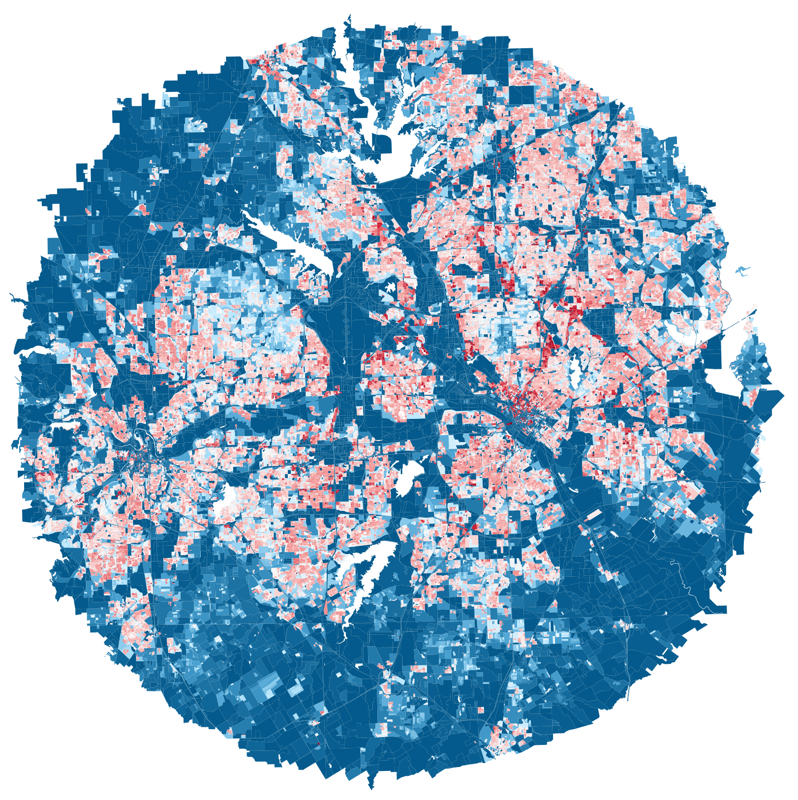
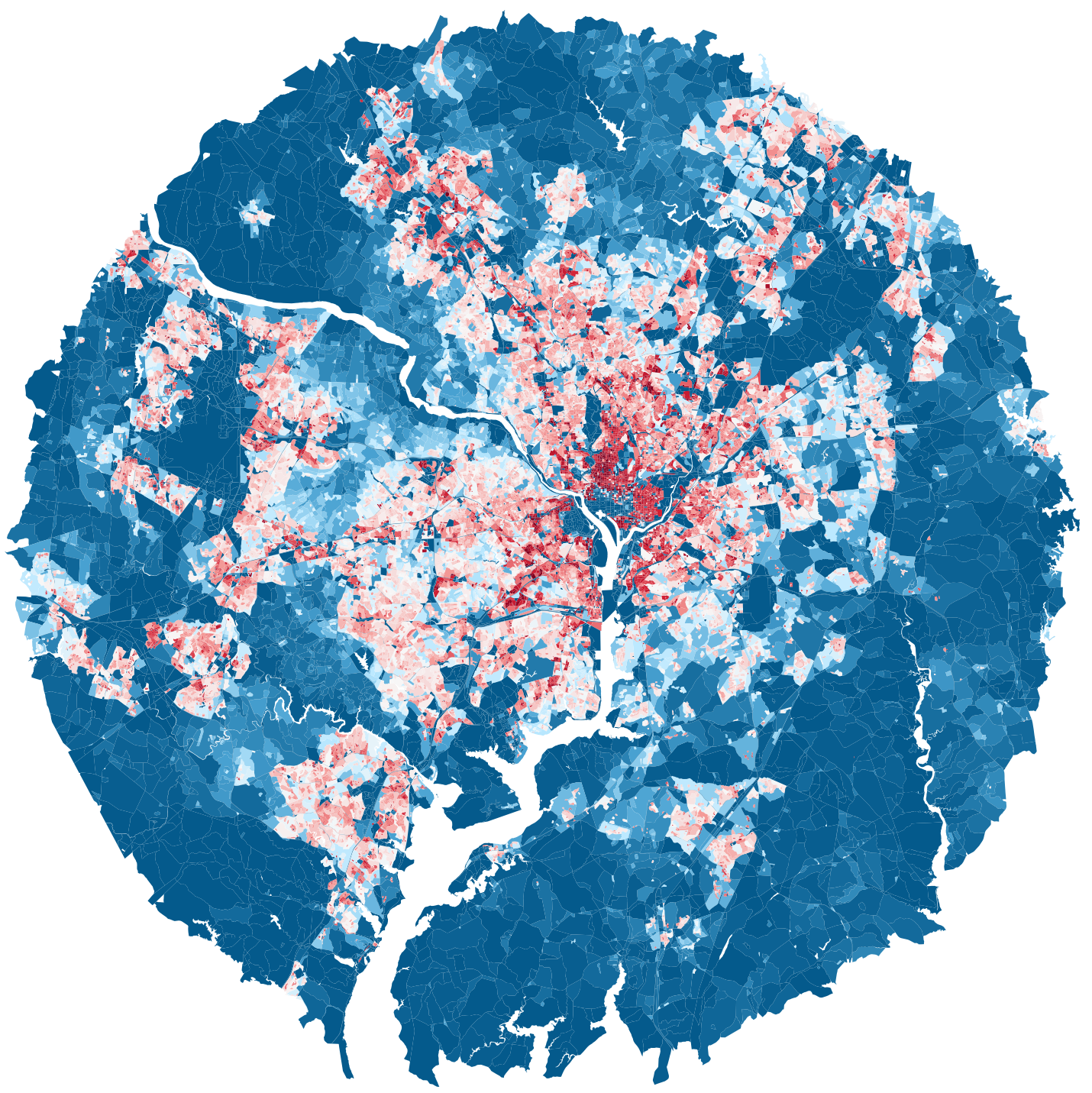
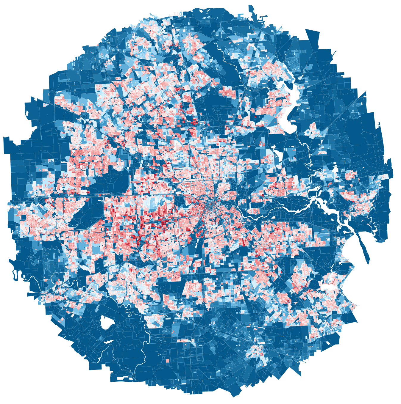
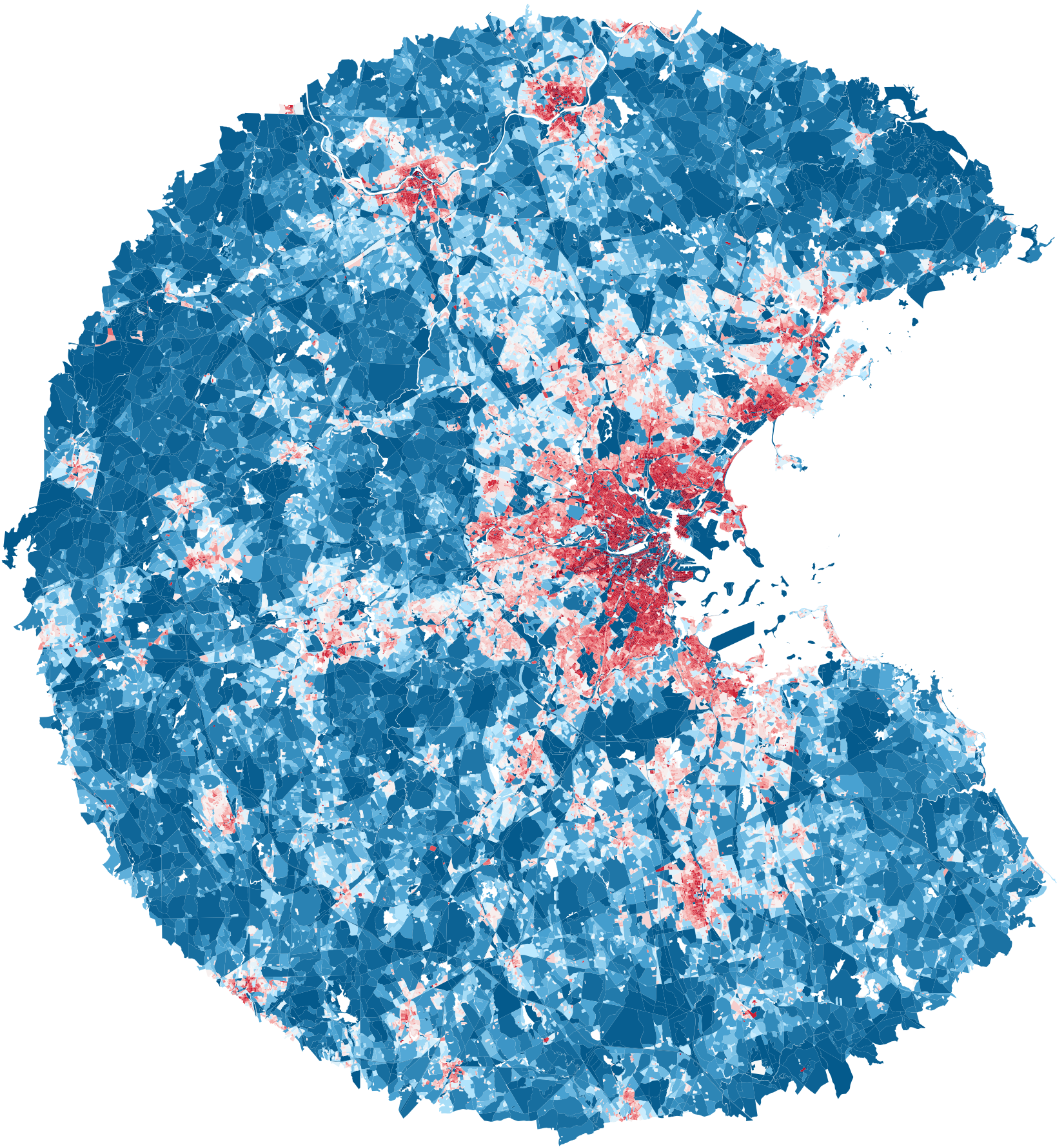
Overview: Top 10 U.S. Cities
Top 10 Cities Population Density Heatmap — by GDP
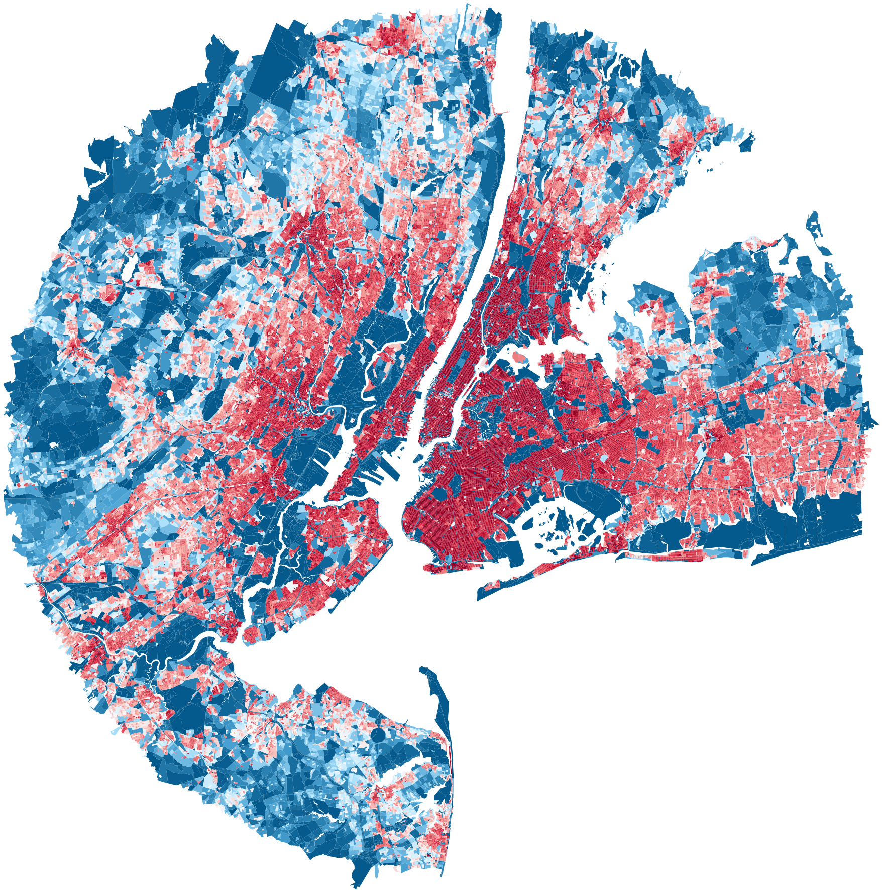
New York City
GDP: 2,298,868 M
population: 19,940,274
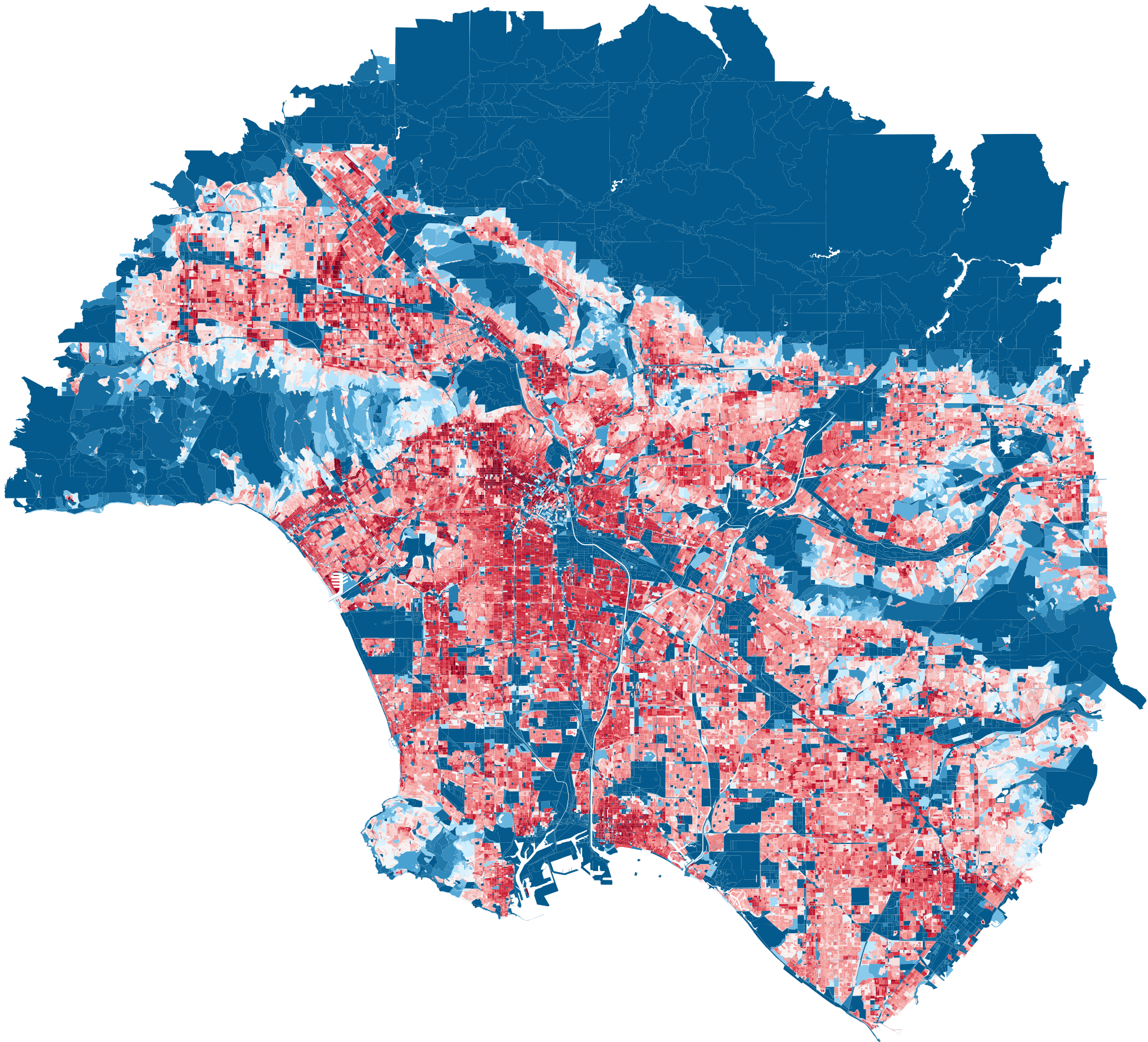
Los Angeles
GDP: 1,295,361 M
population: 12,927,614
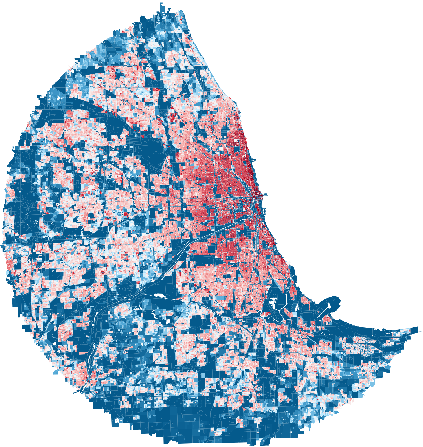
Chicago
GDP: 894,862 M
population: 9,408,576
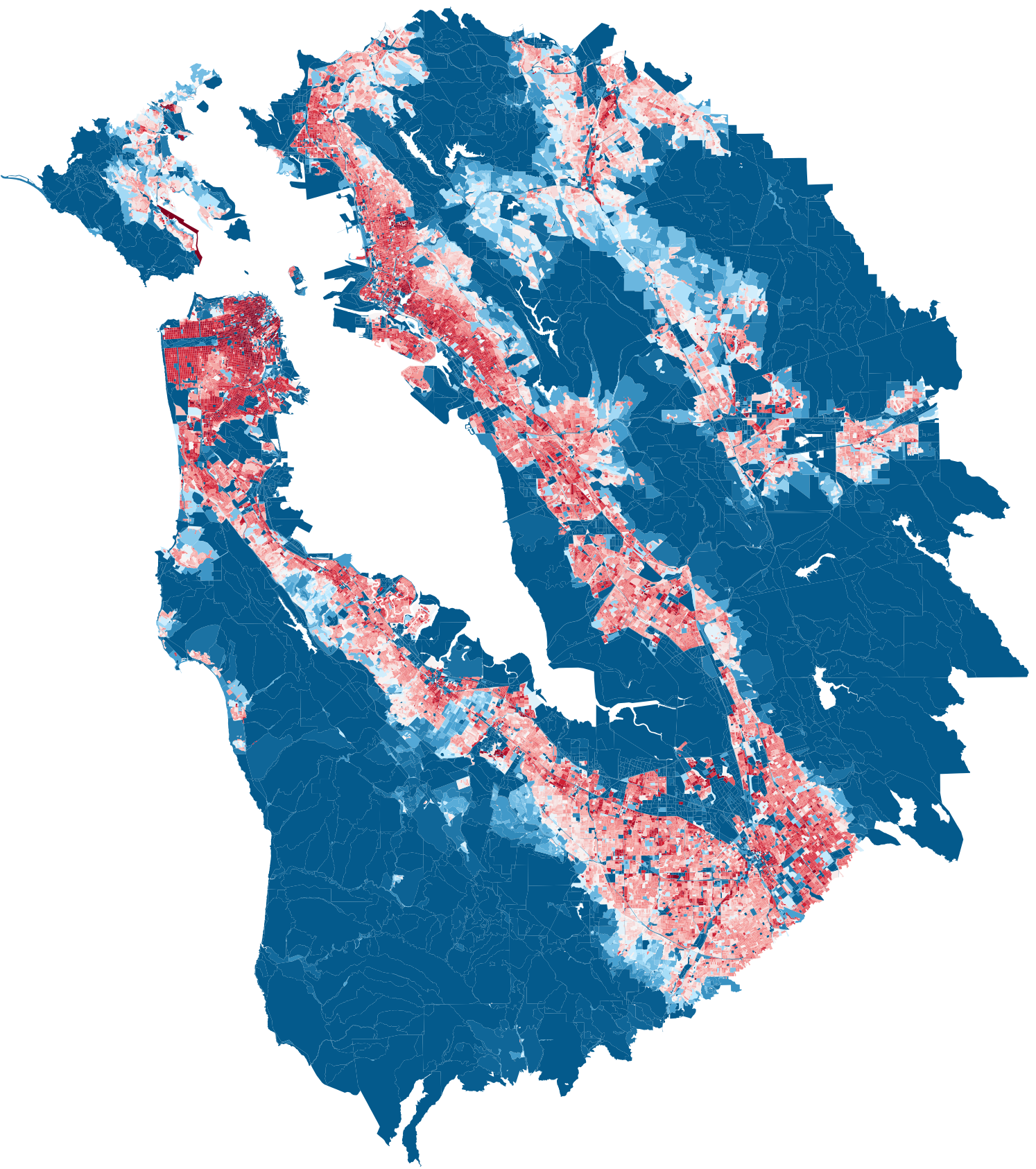
Bay Area
GDP: 778,878 M
population: 4,648,486
Dallas
GDP: 744,654 M
population: 8,344,032
Washington DC
GDP: 714,685 M
population: 6,436,489
Houston
GDP: 696,999 M
population: 7,796,182
Boston
GDP: 610,486 M
population: 5,025,517
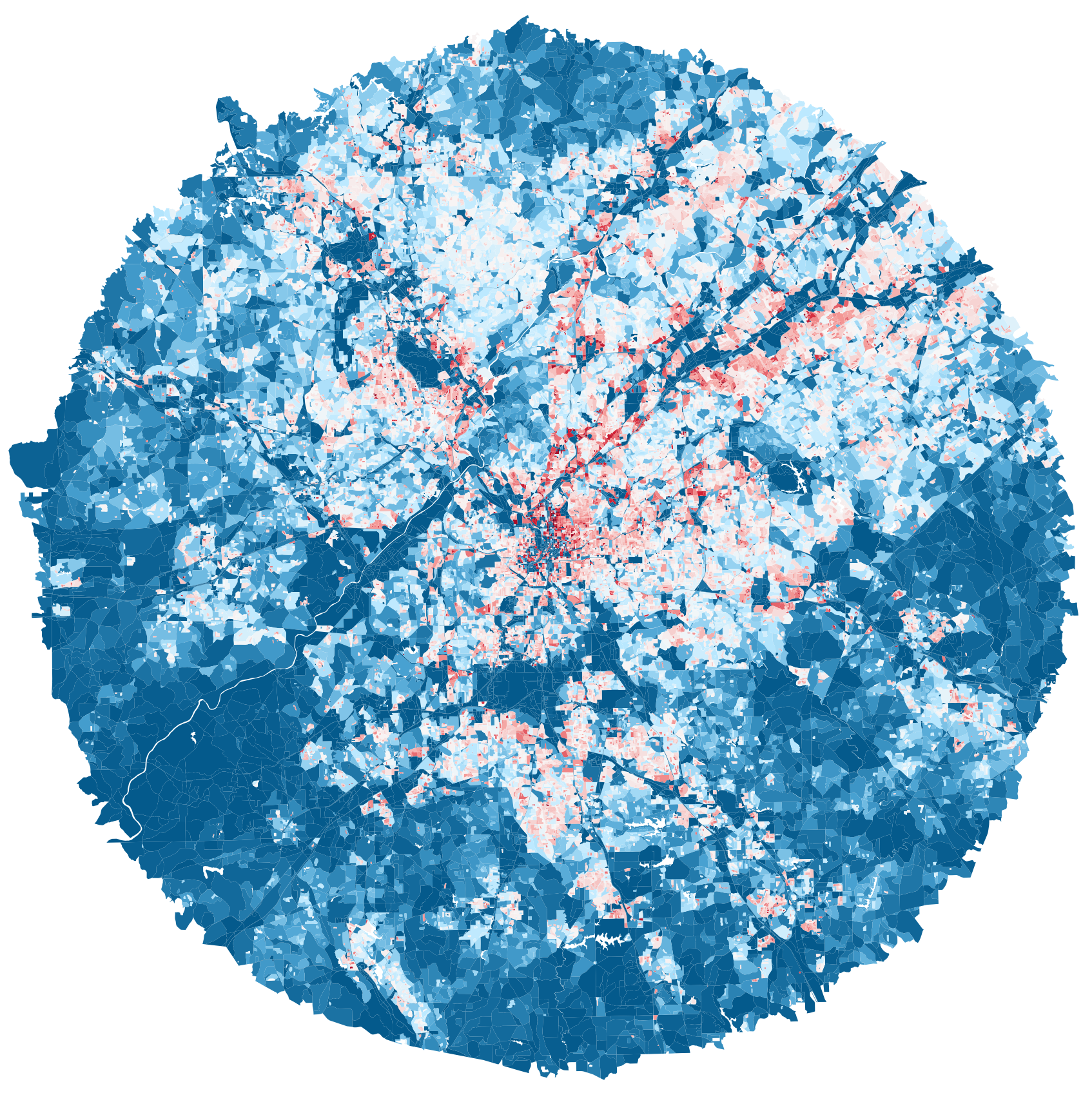
Atlanta
GDP: 570,663 M
population: 6,411,149
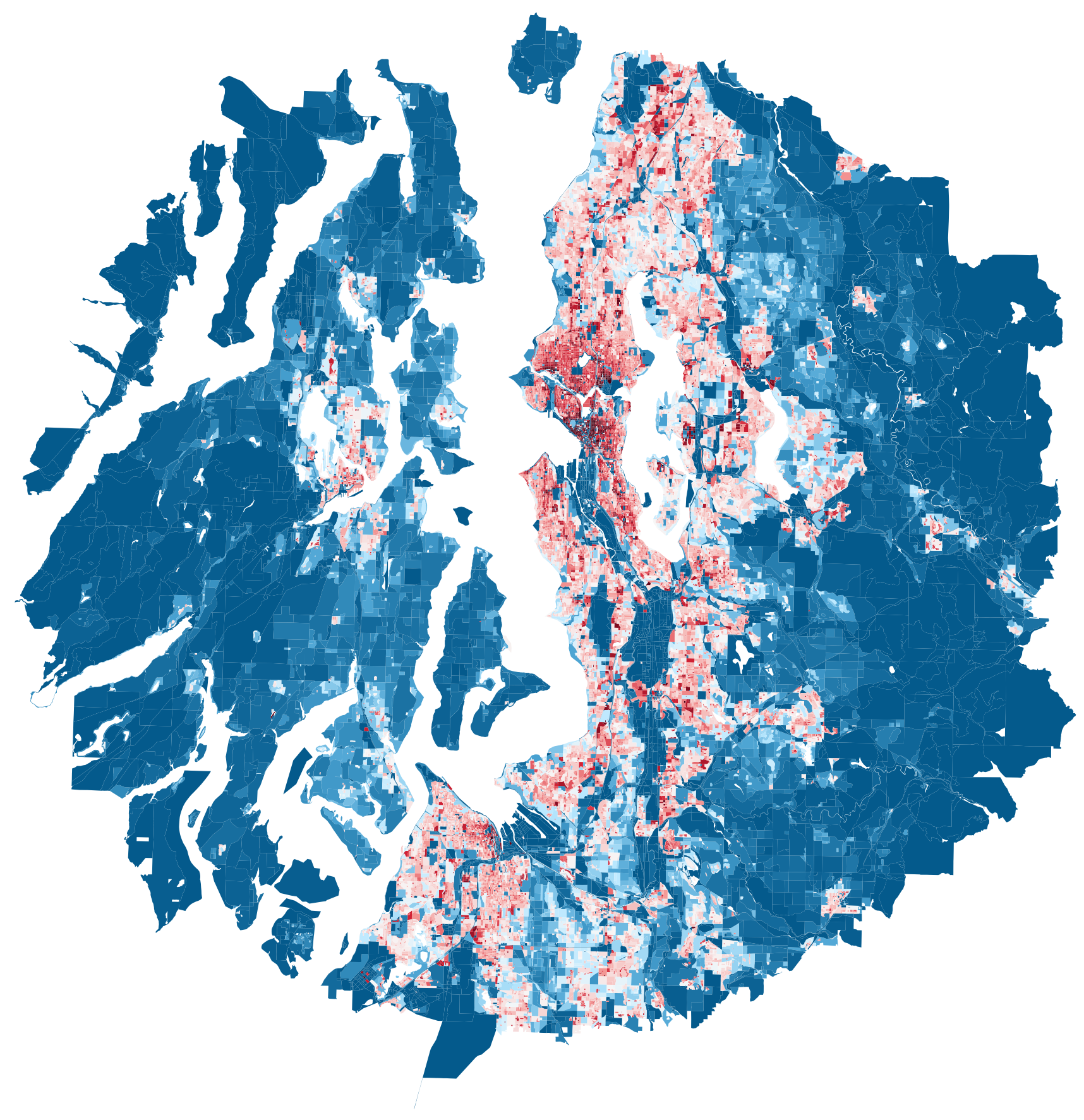
Seattle
GDP: 566,742 M
population: 4,145,494


sample streetblocks
Linear Regression: Geometry as Predictor of Population
Log-transformed linear regression was applied to evaluate whether each of the four geometric features is a meaningful predictor of population density. The analysis was conducted with all 10 cities combined, totaling 746,049 street blocks.
The model was fitted using a logarithmic transformation on the dependent variable, allowing linear regression to capture the exponential relationship between block geometry and density. Scikit-learn's Linear Regression (Ordinary Least Squares, no regularization) was used.
population density = e(β0 + β1 · log(area))
population density = e(β0 + β1 · feature) (Isoperimetric Quotient, Rectangularity, Solidity)
Model applied to each feature independently:

Area
MSE = 0.889 · R² = 0.436 (Moderate)

Isoperimetric Quotient
MSE = 1.499 · R² = 0.048 (Very Weak)

Rectangularity
MSE = 1.382 · R² = 0.123 (Weak)

Solidity
MSE = 1.419 · R² = 0.099 (Weak)
Combined Model
population density = e(β0 + β1·log(area) + β2·IQ + β3·Rectangularity + β4·Solidity)
| Area Coefficient | −631.634 |
| Isoperimetric Quotient Coefficient | −59.216 |
| Rectangularity Coefficient | 163.857 |
| Solidity Coefficient | −91.977 |
| Mean Squared Error | 0.873 |
| R² | 0.446 |
Geometric variables alone explain approximately 44.6% of the variance in log-transformed population density (R² = 0.446). While this is limited relative to the full complexity of urban density — shaped by socioeconomic, infrastructural, and historical factors — it confirms that block geometry captures a statistically meaningful portion of urban form variation correlated with density.
The p-values for all four variables are near zero, confirming that the observed relationships are statistically significant — a finding made reliable by the large sample size of 746,049 street blocks.
Logistic Regression: Geometry as Classifier of Urbanity
The original dataset includes an urbanity indicator (UR20) that classifies each street block as Urban or Rural. This classification, defined by the U.S. Census Bureau, is based on factors such as population density and spatial continuity — not on any geometric attributes. The objective of this analysis is to evaluate whether the four geometric features (Area, Isoperimetric Quotient, Rectangularity, and Solidity) can effectively predict this label.
A logistic regression model was trained on data from all ten metropolitan areas, using bootstrapping and 10-fold cross-validation to ensure robustness and generalization. The trained model was subsequently tested on an unseen city (Philadelphia) to evaluate transferability.
log P(UR20 = 1)1 − P(UR20 = 1) = β0 + β1·area + β2·IQ + β3·rectangularity + β4·solidity
| Intercept (β0) | 3.940 |
| Area (β1) | −1.023 |
| Isoperimetric Quotient (β2) | −0.028 |
| Rectangularity (β3) | −0.330 |
| Solidity (β4) | 0.988 |
| Error Rate (10 training cities) | 0.0299 (97.01% accuracy) |
| Error Rate (Philadelphia, unseen) | 0.0626 (93.74% accuracy) |
The model achieved 97.01% accuracy across the ten training cities and 93.74% accuracy on the unseen city of Philadelphia. These results demonstrate that street-block geometry alone provides a strong predictive basis for distinguishing urban from rural classifications, and that the learned relationships generalize well beyond the training data.

Philadelphia: Predicted Urban vs. Rural Blocks

Philadelphia: Urban vs. Rural Blocks (Ground Truth)
Graph Neural Network
Abstract
This project extends the Street-Block Machine Learning study under the same fundamental premise: how much urban structure can be inferred solely from street-block geometry, independent of socioeconomic or land-use data. Using street-block data from the United States Census Bureau, the study focuses on the top 10 U.S. metropolitan areas by GDP. The ground-truth label is the UR20 attribute, framing the task as a binary classification problem (urban vs. rural).
While the previous ML approach relied on four handcrafted geometric features, this project asks a more fundamental question: can a model learn urbanity directly from raw geometry? Street blocks are represented as graphs derived from polygon topology, and a Graph Neural Network (GNN) is trained to classify urban versus rural blocks based purely on learned geometric representations. By replacing feature engineering with end-to-end geometric learning, the project evaluates the expressive limits of deep learning for urban form inference and clarifies what information is intrinsically embedded in street-block geometry alone.
Workflow
QGIS: Loaded shapefiles, clipped to a 30-mile radius per city, calculated base geometric attributes, and exported processed layers.
PostgreSQL/PostGIS: Stored city-wise processed street-block geometries and UR20 labels, enabling consistent querying and reproducible splits.
Python + PyTorch Geometric: Loaded all 10 cities, converted blocks into graph representations, trained a GNN on 9 cities with Houston as a fixed validation set, and tested generalization on an unseen city: Philadelphia.

Street Block to Graph
Street blocks can be modeled either as rasterized images or as graphs. An image representation forces a grid-based approximation and often loses precise corner-to-corner structure, while a graph preserves the true topology of the polygon — capturing explicit relationships between corners (nodes) and edges (connections).
Each street block is converted into a planar graph where polygon vertices become nodes and consecutive boundary segments become edges. Node features are stored in an N × 5 matrix, where each of the N vertices contains five attributes: (x, y) coordinates, turning angle θ at the vertex, and the lengths of the two adjacent boundary edges (l1, l2).
The conversion pipeline standardizes vertex ordering, removes duplicate and near-duplicate points, computes angles and edge lengths from the cleaned polygon boundary, builds the edge index from sequential vertex connectivity (including wrap-around from last to first vertex), and outputs a graph object: x ∈ ℝN×5 and edge_index ∈ ℕ2×E.
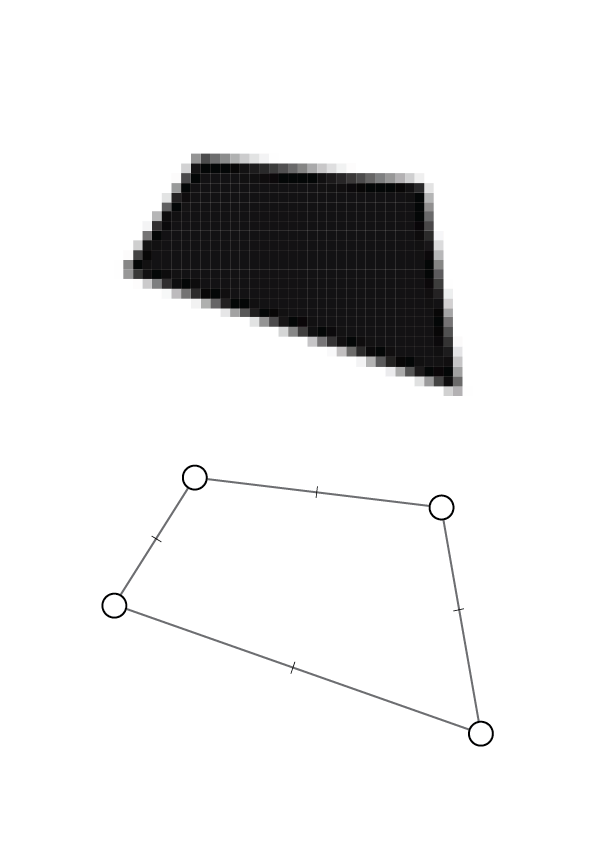
Image vs. Graph representation of a street block
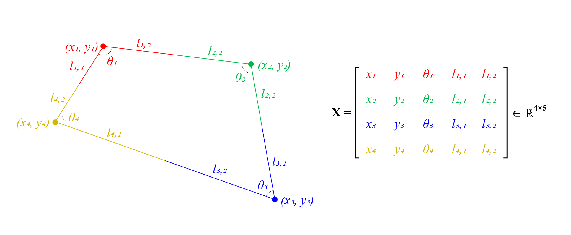
Sample graph structure (x, y, θ, l1, l2)
Neural Network Iterations
The deep learning model is built around a GNN that learns hierarchical geometric representations of street-block graphs. Two architectural configurations were tested to evaluate the effect of model capacity on generalization.
Iteration 1 — Node embeddings are projected through a graph convolution layer into a 64-dimensional latent space, followed by global pooling and a multilayer perceptron (MLP) for binary classification:
Graph Conv → N × 64 → Global Pooling → MLP: 64 → 128 → 256 → 1
Iteration 2 — Model capacity is increased to test whether richer geometric abstractions improve generalization. The convolution output is expanded to 128 dimensions, and the MLP uses a deeper but uniform architecture:
Graph Conv → N × 128 → Global Pooling → MLP: 128 → 128 → 128 → 128 → 1
Across both iterations, the network is trained end-to-end using supervised learning with a binary classification objective. This iterative setup enables a direct comparison between compact and high-capacity architectures, clarifying the trade-off between expressiveness and overfitting when learning urban form purely from geometry.
Neural Network Architecture

Treating Imbalanced Data

The dataset exhibits severe class imbalance: urban blocks account for approximately 98% of all street blocks by count, while rural blocks represent a small minority. However, when evaluated by total area, the imbalance is less extreme — urban blocks cover roughly twice the area of rural blocks, reflecting the much larger spatial footprint of rural street blocks. Block count alone is therefore a misleading indicator of spatial dominance.
Synthetic oversampling methods such as SMOTE were intentionally not used. Street-block geometry is highly sensitive to small perturbations, and generating synthetic samples risks producing geometries that are topologically invalid or physically implausible — corrupting the learning signal in a graph-based model.
Instead, class imbalance is addressed through area-based loss weighting, so that misclassification penalties are proportional to the spatial footprint of each block rather than raw sample counts. This aligns the optimization objective with spatial reality, reduces bias toward over-predicting the majority urban class, and preserves the integrity of original geometries. By decoupling data representation from error weighting, the model maintains consistent graph inputs while correcting imbalance at the learning stage — enabling more meaningful generalization to unseen cities.
Conclusion

The deep learning approach achieves 94.55% accuracy, only marginally improving over the 93.74% accuracy obtained from the logistic regression model. A closer examination of the confusion matrices reveals where this difference originates. Logistic regression strongly favors the majority class, predicting urban blocks far more aggressively due to the overwhelming count imbalance. This results in very high urban recall but poor rural recognition, with many rural blocks incorrectly classified as urban.

Logistic Regression Confusion Matrix

Neural Network (GNN) Confusion Matrix
The GNN demonstrates a more balanced error distribution. While overall accuracy gains are modest, the network improves both precision and recall for the minority rural class — reducing false urban predictions and yielding a cleaner separation between urban and rural blocks. This indicates that the GNN is better at extracting subtle geometric signals that distinguish large rural blocks from dense urban fabrics, even under severe class imbalance.
Despite this improvement, the results expose a clear limitation. Across 50 training epochs and both architectural iterations, the loss and error rate plateau after approximately 20 epochs without further meaningful improvement. This suggests that street-block geometry alone has bounded explanatory power for urban classification. While the GNN is more expressive than logistic regression, it is also less efficient and more computationally expensive, delivering only incremental gains. The outcome implies that deep learning does not fundamentally overcome the information ceiling imposed by geometry-only inputs — rather, it slightly refines classification within those limits. This reinforces the conclusion that urbanity is only partially encoded in block shape, and that richer contextual or semantic data would be required for significant performance gains beyond this threshold.

Ambiguous street block geometric patterns: Suburb New Jersey

Ambiguous street block geometric patterns: Bay Area